Supervised Training#
We will first target a “purely” data-driven approach, in line with classic machine learning. We’ll refer to this as a supervised approach in the following, to indicate that the network is fully supervised by data, and to distinguish it from using physics-based losses. One of the central advantages of the supervised approach is that we obtain a surrogate model (also called “emulator”, or “Neural operator”), i.e., a new function that mimics the behavior of the original \(\mathcal{P}\).
The purely data-driven, supervised training is the central starting point for all projects in the context of deep learning. While it can yield suboptimal results compared to approaches that more tightly couple with physics, it can be the only choice in certain application scenarios where no good model equations exist. In this chapter, we’ll also go over the basics of different neural network architectures. Next to training methodology, this is an imporant choice.
Problem setting#
For supervised training, we’re faced with an unknown function \(f^*(x)=y^*\), collect lots of pairs of data \([x_0,y^*_0], ...[x_n,y^*_n]\) (the training data set) and directly train an NN to represent an approximation of \(f^*\) denoted as \(f\).
The \(f\) we can obtain in this way is typically not exact, but instead we obtain it via a minimization problem: by adjusting the weights \(\theta\) of our NN representation of \(f\) such that we minimize the error over all data points in the training set
This will give us \(\theta\) such that \(f(x;\theta) = y \approx y^*\) as accurately as possible given our choice of \(f\) and the hyperparameters chosen for training. Note that above we’ve assumed the simplest case of an \(L^2\) loss. A more general version would use an error metric \(e(x,y)\) in the loss \(L\) to be minimized via \(\text{arg min}_{\theta} \sum_i e( f(x_i ; \theta) , y^*_i) )\). The choice of a suitable metric is a topic we will get back to later on. The minimization above constitutes the actual “learning” process, and is non-trivial because \(f\) is usually a non-linear function.
The training data typically needs to be of substantial size, and hence it is attractive to use numerical simulations solving a physical model \(\mathcal{P}\) to produce a large number of reliable input-output pairs for training. This means that the training process uses a set of model equations, and approximates them numerically, in order to fit the NN representation \(f\). This has quite a few advantages, e.g., we don’t have the measurement noise of real-world devices and we don’t need manual labour to annotate a large number of samples to get training data.
On the other hand, this approach inherits the common challenges of replacing experiments with simulations: first, we need to ensure the chosen model has enough power to predict the behavior of the simulated phenomena that we’re interested in. In addition, the numerical approximations have numerical errors which need to be kept small enough for a chosen application (otherwise even the best NN has no chance to be provide a useful answer later on). As these topics are studied in depth for classical simulations, and the existing knowledge can likewise be leveraged to set up DL training tasks.
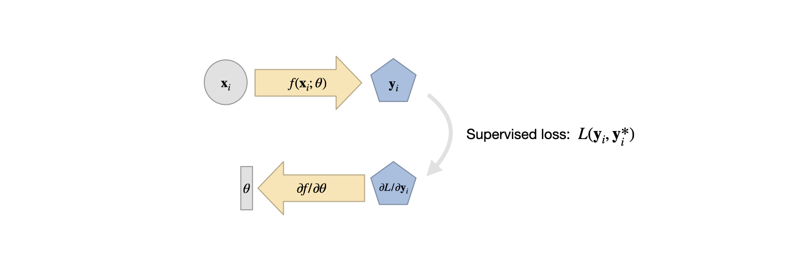
Fig. 5 A visual overview of supervised training. It’s simple, and a good starting point in comparison to the more complex variants we’ll encounter later on.#
Looking ahead#
The numerical approximations of PDE models for real world phenomena are often very expensive to compute. A trained NN on the other hand incurs a constant cost per evaluation, and is typically trivial to evaluate on specialized hardware such as GPUs or NN compute units.
Despite this, it’s important to be careful: NNs can quickly generate huge numbers of in between results. Consider a CNN layer with \(128\) features. If we apply it to an input of \(128^2\), i.e. ca. 16k cells, we get \(128^3\) intermediate values. That’s more than 2 million. All these values at least need to be momentarily stored in memory, and processed by the next layer. Nonetheless, replacing complex and expensive solvers with fast, learned approximations is a very attractive and interesting direction.
An important decision to make at this stage is which neural network architecture to choose.