Unstructured Meshes and Meshless Methods#
For all computer-based methods we need to find a suitable discrete representation. While this is straight-forward for cases such as data consisting only of integers, it is more challenging for continuously changing quantities such as the temperature in a room. While the previous examples have focused on aspects beyond discretization (and used Cartesian grids as a placeholder), the following chapter will target scenarios where learning Neural operators with dynamically changing and adaptive discretizations have a benefit.
Types of computational meshes#
As outlined in Neural Network Architectures, we can distinguish three types of computational meshes (or “grids”) with which discretizations are typically performed:
structured meshes: Structured meshes have a regular arrangement of the sample points, and an implicitly defined connectivity. In the simplest case it’s a dense Cartesian grid.
unstructured meshes: On the other hand can have an arbitrary connectivity and arrangement. The flexibility gained from this typically also leads to an increased computational cost.
meshless or particle-based finally share arbitrary arrangements of the sample points with unstructured meshes, but in contrast implicitly define connectivity via neighborhoods, i.e. a suitable distance metric.
Structured meshes are currently very well supported within DL algorithms due to their similarity to image data, and hence they typically simplify implementations and allow for using stable, established DL components (especially regular convolutional layers). However, for target functions that exhibit an uneven mix of smooth and complex regions, the other two mesh types can have advantages.
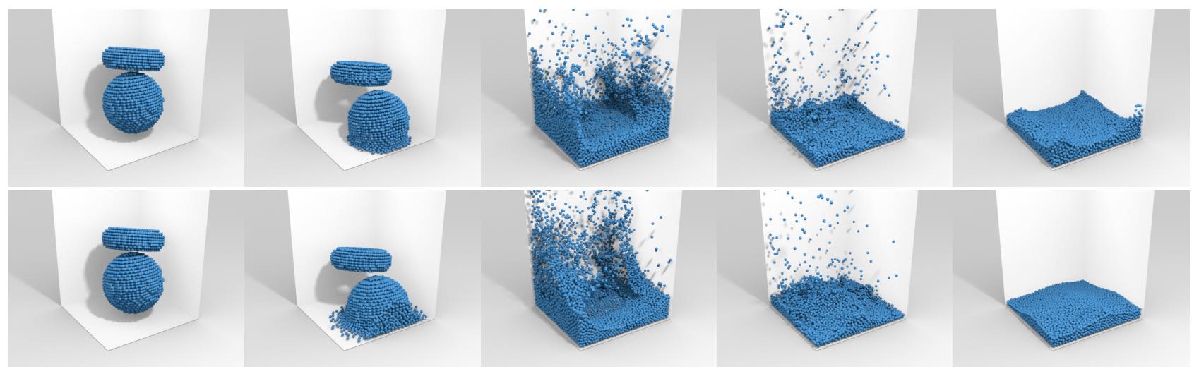
Fig. 60 Lagrangian simulations of liquids: the sampling points move with the material, and undergo large changes. In the top row timesteps of a learned simulation, in the bottom row the traditional SPH solver.#
Unstructured meshes and graph neural networks#
Within computational sciences the generation of improved mesh structures is a challenging and ongoing effort. The numerous H-,C- and O-type meshes which were proposed with numerous variations over the years for flows around airfoils are a good example.
Unstructured meshes offer the largest flexibility here on the meshing side, but of course need to be supported by the simulator. Interestingly, unstructured meshes share many properties with graph neural networks (GNNs), which extend the classic ideas of DL on Cartesian grids to graph structures. Despite growing support, working with GNNs typically causes a fair amount of additional complexity in an implementation, and the arbitrary connectivities call for message-passing approaches between the nodes of a graph. This message passing is usually realized using fully-connected layers, instead of convolutions.
Thus, in the following, we will focus on a particle-based method [UPTK19], which offers the same flexibility in terms of spatial adaptivity as GNNs. These were previously employed for a very similar goal [SGGP+20], however, the method below enables a real convolution operator for learning the physical relationships.
Meshless and particle-based methods#
Organizing connectivity explicitly is particularly challenging in dynamic cases, e.g., for Lagrangian representations of moving materials where the connectivity quickly becomes obsolete over time. In such situations, methods that rely on flexible, re-computed connectivities are a good choice. Operations are then defined in terms of a spatial neighborhood around the sampling locations (also called “particles” or just “points”), and due to the lack of an explicit mesh-structure these methods are also known as “meshless” methods. Arguably, different unstructured, graph and meshless variants can typically be translated from one to the other, but nonetheless the rough distinction outlined above gives an indicator for how a method works.
In the following, we will discuss an example targeting splashing liquids as a particularly challenging case. For these simulations, the fluid material moves significantly and is often distributed very non-uniformly.
The general outline of a learned, particle-based simulation is similar to a DL method working on a Cartesian grid: we store data such as the velocity at certain locations, and then repeatedly perform convolutions to create a latent space at each location. Each convolution reads in the latent space content within its support and produces a result, which is activated with a suitable non-linear function such as ReLU. This is done multiple times in parallel to produce a latent space vector, and the resulting latent space vectors at each location serve as inputs for the next stage of convolutions. After expanding the size of the latent space over the course of a few layers, it is contracted again to produce the desired result, e.g., an acceleration.
Continuous convolutions#
A generic, discrete convolution operator to compute the convolution \((f*g)\) between functions \(f\) and \(g\) has the form
where \(\tau\) denotes the offset vector, and \(\Omega\) defines the support of the filter function (typically \(g\)).
We transfer this idea to particles and point clouds by evaluating a convolution on a set of \(i\) locations \(\mathbf{x}_i\) in a radial neighborhood \(\mathcal N(\mathbf{x}, R)\) around \(\mathbf{x}\). Here, \(R\) denotes the radius within which the convolution should have support. We define a continuous version of the convolution following [UPTK19]:
Here, the mapping \(\Lambda\) plays a central role: it represents a mapping from the unit ball to the unit cube, which allows us to use a simple grid to represent the unknowns in the convolution kernel. This greatly simplifies the construction and handling of the convolution kernel, and is illustrated in the following figure:
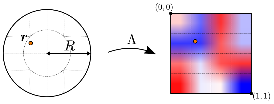
Fig. 61 The unit ball to unit cube mapping employed for the kernel function of the continuous convolution.#
In a physical setting, e.g., the simulation of fluid dynamics, we can additionally introduce a radial weighting function, denoted as \(a\) below to make sure the kernel has a smooth falloff. This yields
where \(a_{\mathcal N}\) denotes a normalization factor \(a_{\mathcal N} = \sum_{i \in \mathcal N(\mathbf{x}, R)} a(\mathbf{x}_i, \mathbf{x})\). There’s is quite some flexibility for \(a\), but below we’ll use the following weighting function
This ensures that the learned influence smoothly drops to zero for each of the individual convolutions.
For a lean architecture, a small fully-connected layer can be added for each convolution to process the content of the destination particle itself. This makes it possible to use relatively small kernels with even sizes, e.g., sizes of \(4^3\) [UPTK19].
Learning the dynamics of liquids#
The architecture outlined above can then be trained with a collection of randomized reference data from a particle-based Navier-Stokes solver. The resulting network yields a good accuracy with a very small and efficient model. E.g., compared to GNN-based approaches the continuous convolution requires significantly fewer weights and is faster to evaluate.
Interestingly, a particularly tough case for such a learned solver is a container of liquid that should come to rest. If the training data is not specifically engineered to contain many such cases, the network receives only a relatively small of such cases at training time. Moreover, a simulation typically takes many steps to come to rest (many more than are unrolled for training). Hence the network is not explicitly trained to reproduce such behavior.
Nonetheless, an interesting side-effect of having a trained NN for such a liquid simulation by construction provides a differentiable solver. Based on a pre-trained network, the learned solver then supports optimization via gradient descent, e.g., w.r.t. input parameters such as viscosity. The following image shows an examplary prediction task with continuous convolutions from [UPTK19].
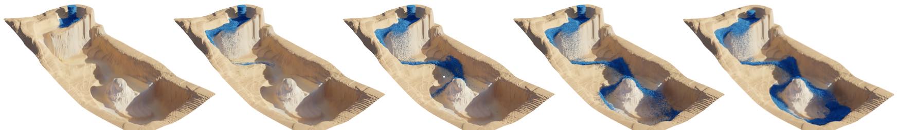
Fig. 62 An example of a particle-based liquid spreading in a landscape scenario, simulated with learned, continuous convolutions.#
Source code#
For a practical implementation of the continuous convolutions, another important step is a fast collection of neighboring particles for \(\mathcal N\). An efficient example implementation can be found at intel-isl/DeepLagrangianFluids, together with training code for learning the dynamics of liquids, an example of which is shown in the figure above.