Overview#
The name of this book, Physics-Based Deep Learning, denotes combinations of physical modeling and numerical simulations with methods based on artificial intelligence, i.e. neural networks. The general direction of Physics-Based Deep Learning, also going under the name Scientific Machine Learning, represents a very active, quickly growing and exciting field of research. The following chapter will give a more thorough introduction to the topic and establish the basics for following chapters.

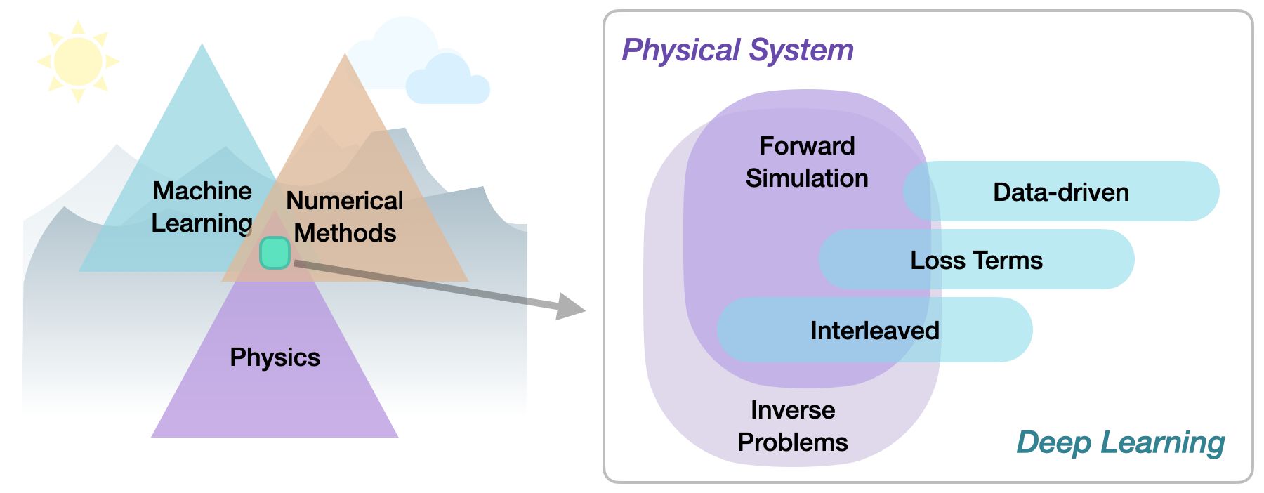
Fig. 4 Understanding our environment, and predicting how it will evolve is one of the key challenges of humankind. A key tool for achieving these goals are computer simulations, and the next generation of these simulations will likely strongly profit from integrating AI and deep learning components, in order to make even better accurate predictions about the phenomena in our environment.#
Motivation#
From weather and climate forecasts [Sto14] (see the picture above), over quantum physics [OMalleyBK+16], to the control of plasma fusion [MLA+19], using numerical analysis to obtain solutions for physical models has become an integral part of science.
In recent years, artificial intelligence driven by deep neural networks, have led to impressive achievements in a variety of fields: from image classification [KSH12] over natural language processing [RWC+19], and protein folding [Qur19], to various foundation models. The field is very vibrant and quickly developing, with the promise of vast possibilities.
Replacing traditional simulations?#
These success stories of deep learning (DL) approaches have given rise to concerns that this technology has the potential to replace the traditional, simulation-driven approach to science. E.g., recent works show that NN-based surrogate models achieve accuracies required for real-world, industrial applications such as airfoil flows [CT22], while at the same time outperforming traditional solvers by orders of magnitude in terms of runtime.
Instead of relying on models that are carefully crafted from first principles, can sufficiently large datasets be processed instead to provide the correct answers? As we’ll show in the next chapters, this concern is unfounded. Rather, it is crucial for the next generation of simulation systems to bridge both worlds: to combine classical numerical techniques with A.I. methods. In addition, the latter offer exciting new possibilities in areas that have been challenging for traditional methods, such as dealing with complex distributions and uncertainty in simulations.
One central reason for the importance of the combination with numerics is that DL approaches are powerful, but at the same time strongly profit from domain knowledge in the form of physical models. DL techniques and NNs are novel, sometimes difficult to apply, and it is admittedly often non-trivial to properly integrate our understanding of physical processes into the learning algorithms.
Over the last decades, highly specialized and accurate discretization schemes have been developed to solve fundamental model equations such as the Navier-Stokes, Maxwell’s, or Schroedinger’s equations. Seemingly trivial changes to the discretization can determine whether key phenomena are visible in the solutions or not. Rather than discarding the powerful methods that have been developed in the field of numerical mathematics, this book will show that it is highly beneficial to use them as much as possible when applying DL.
Black boxes?#
In the past, AI and DL methods have often associated trained neural networks with black boxes, implying that they are something that is beyond the grasp of human understanding. However, these viewpoints typically stem from relying on hearsay and general skepticism about “hyped” topics.
The situation is a very common one in science, though: we are facing a new class of methods, and “all the gritty details” are not yet fully worked out. This is and has been pretty common for all kinds of scientific advances. Numerical methods themselves are a good example. Around 1950, numerical approximations and solvers had a tough standing. E.g., to cite H. Goldstine, numerical instabilities were considered to be a “constant source of anxiety in the future” [Gol90]. By now we have a pretty good grasp of these instabilities, and numerical methods are ubiquitous and well established. AI, neural networks follow the same path of human progress.
Thus, it is important to be aware of the fact that – in a way – there is nothing very special or otherworldly to deep learning methods. They’re simply a new set of numerical tools. That being said, they’re clearly very new, and right now definitely the most powerful set of tools we have for non-linear problems. That all the details aren’t fully worked out and have nicely been written up shouldn’t stop us from including these powerful methods in our numerical toolbox.
Reconciling AI and simulations#
Taking a step back, the aim of this book is to build on all the powerful techniques that we have at our disposal for numerical simulations, and use them wherever we can in conjunction with deep learning. As such, a central goal is to reconcile the AI viewpoint with physical simulations.
Goals of this document
The key aspects that we will address in the following are:
how to use deep learning techniques to solve PDE problems,
how to combine them with existing knowledge of physics,
without discarding numerical methods.
At the same time, it’s worth noting what we won’t be covering:
there’s no in-depth introduction to deep learning and numerical simulations (there are great other works already taking care of this),
and the aim is neither a broad survey of research articles in this area.
The resulting methods have a huge potential to improve what can be done with numerical methods: in scenarios where a solver targets cases from a certain well-defined problem domain repeatedly, it can for instance make a lot of sense to once invest significant resources to train a neural network that supports the repeated solves. The development of large so-called “foundation models” is especially promising in this area. Based on the domain-specific specialization via fine-tuning with a smaller dataset, a hybrid solver could vastly outperform traditional, generic solvers. And despite the many open questions, first publications have demonstrated that this goal is a realistic one [KSA+21, UBH+20].
Another way to look at it is that all mathematical models of our nature are idealized approximations and contain errors. A lot of effort has been made to obtain very good model equations, but to make the next big step forward, AI and DL methods offer a very powerful tool to close the remaining gap towards reality [AAC+19].
Categorization#
Within the area of physics-based deep learning, we can distinguish a variety of different approaches, e.g., targeting constraints, combined methods, optimizations and applications. More specifically, all approaches either target forward simulations (predicting state or temporal evolution) or inverse problems (e.g., obtaining a parametrization or state for a physical system from observations).
No matter whether we’re considering forward or inverse problems, the most crucial differentiation for the following topics lies in the nature of the integration between DL techniques and the domain knowledge, typically in the form of model equations via partial differential equations (PDEs). The following three categories can be identified to roughly categorize physics-based deep learning (PBDL) techniques:
Supervised: the data is produced by a physical system (real or simulated), but no further interaction exists. This is the classic machine learning approach.
Loss-terms: the physical dynamics (or parts thereof) are encoded in the loss function, typically in the form of differentiable operations. The learning process can repeatedly evaluate the loss, and usually receives gradients from a PDE-based formulation. These soft constraints sometimes also go under the name “physics-informed” training.
Hybrid: the full physical simulation is interleaved and combined with an output from a deep neural network; this usually requires a fully differentiable simulator. It represents the tightest coupling between the physical system and the learning process and results in a hybrid solver that combines classic techniques with AI-based ones.
Thus, methods can be categorized in terms of forward versus inverse solve, and how tightly the physical model is integrated with the neural network. Here, especially hybrid approaches that leverage differentiable physics allow for very tight integration of deep learning and numerical simulation methods.
Naming#
It’s worth pointing out that what we’ll call “differentiable physics” in the following appears under a variety of different names in other resources and research papers. The differentiable physics name is motivated by the differentiable programming paradigm in deep learning. Here we, e.g., also have “differentiable rendering approaches”, which deal with simulating how light leads forms the images we see as humans. In contrast, we’ll focus on physical simulations from now on, hence the name.
When coming from other backgrounds, other names are more common however. E.g., the differentiable physics approach is equivalent to using the adjoint method, and coupling it with a deep learning procedure. Effectively, it is also equivalent to apply backpropagation / reverse-mode differentiation to a numerical simulation. However, as mentioned above, motivated by the deep learning viewpoint, we’ll refer to all these as “differentiable physics” approaches from now on.
The hybrid solvers that result from integrating DL with a traditional solver can also be seen as a classic topic: in this context, the neural network has the task to correct the solver. This correction can in turn either target numerical errors, or unresolved terms in an equation. This is a fundamental problem in science that has been addressed under various names, e.g., as the closure problem in fluid dynamics and turbulence, as homogenization or coarse-graining in material science, and parametrization in climate and weather simulation. The re-invention of this goal in the different fields points to the importance of the underlying problem, and this text will illustrate the new ways that DL offers to tackle it.
Looking ahead#
Physics simulations are a huge field, and we won’t be able to cover all possible types of physical models and simulations.
Note
Rather, the focus of this book lies on:
Dense field-based simulations (no Lagrangian methods)
Combinations with deep learning (plenty of other interesting ML techniques exist, but won’t be discussed here)
Experiments are left as an outlook (i.e., replacing synthetic data with real-world observations)
It’s also worth noting that we’re starting to build the methods from some very fundamental building blocks. Here are some considerations for skipping ahead to the later chapters.
Hint: You can skip ahead if…
you’re very familiar with numerical methods and PDE solvers, and want to get started with DL topics right away. The Supervised Training chapter is a good starting point then.
On the other hand, if you’re already deep into NNs&Co, and you’d like to skip ahead to the research related topics, we recommend starting in the Physical Loss Terms chapter, which lays the foundations for the next chapters.
A brief look at our notation in the Notation and Abbreviations chapter won’t hurt in both cases, though!
Implementations#
This text also represents an introduction to deep learning and simulation APIs. We’ll primarily use the popular deep learning API pytorch https://pytorch.org, but also a bit of tensorflow https://www.tensorflow.org, and additionally give introductions into the differentiable simulation framework ΦFlow (phiflow) tum-pbs/PhiFlow. Some examples also use JAX google/jax, which provides an interesting alternative. Thus after going through these examples, you should have a good overview of what’s available in current APIs, such that the best one can be selected for new tasks.
As we’re dealing with stochastic optimizations in most of the Jupyter notebooks, many of the following code examples will produce slightly different results each time they’re run. This is fairly common with NN training, but it’s important to keep in mind when executing the code. It also means that the numbers discussed in the text might not exactly match the numbers you’ll see after re-running the examples.