Model Reduction and Time Series#
An inherent challenge for many practical PDE solvers is the large dimensionality of the resulting problems. Our model \(\mathcal{P}\) is typically discretized with \(\mathcal{O}(n^3)\) samples for a 3 dimensional problem (with \(n\) denoting the number of samples along one axis), and for time-dependent phenomena we additionally have a discretization along time. The latter typically scales in accordance to the spatial dimensions. This gives an overall samples count on the order of \(\mathcal{O}(n^4)\). Not surprisingly, the workload in these situations quickly explodes for larger \(n\) (and for all practical high-fidelity applications we want \(n\) to be as large as possible).
One popular way to reduce the complexity is to map a spatial state of our system \(\mathbf{s_t} \in \mathbb{R}^{n^3}\) into a much lower dimensional state \(\mathbf{c_t} \in \mathbb{R}^{m}\), with \(m \ll n^3\). Within this latent space, we estimate the evolution of our system by inferring a new state \(\mathbf{c_{t+1}}\), which we then decode to obtain \(\mathbf{s_{t+1}}\). In order for this to work, it’s crucial that we can choose \(m\) large enough that it captures all important structures in our solution manifold, and that the time prediction of \(\mathbf{c_{t+1}}\) can be computed efficiently, such that we obtain a gain in performance despite the additional encoding and decoding steps. In practice, the explosion in terms of unknowns for regular simulations (the \(\mathcal{O}(n^3)\) above) coupled with a super-linear complexity for computing a new state \(\mathbf{s_t}\) directly makes this approach very expensive, while working with the latent space points \(\mathbf{c}\) very quickly pays off for small \(m\).
However, it’s crucial that encoder and decoder do a good job at reducing the dimensionality of the problem. This is a very good task for DL approaches. Furthermore, we then need a time evolution of the latent space states \(\mathbf{c}\), and for most practical model equations, we cannot find closed form solutions to evolve \(\mathbf{c}\). Hence, this likewise poses a very good problem for DL. To summarize, we’re facing two challenges: learning a good spatial encoding and decoding, together with learning an accurate time evolution. Below, we will describe an approach to solve this problem following Wiewel et al. [WBT19] & [WKA+20], which in turn employs the encoder/decoder of Kim et al. [KAT+19].
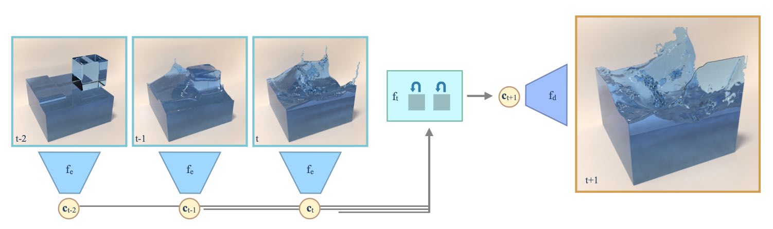
Fig. 58 For time series predictions with ROMs, we encode the state of our system with an encoder \(f_e\), predict the time evolution with \(f_t\), and then decode the full spatial information with a decoder \(f_d\).#
Reduced order models#
Reducing the dimension and complexity of computational models, often called reduced order modeling (ROM) or model reduction, is a classic topic in the computational field. Traditional techniques often employ techniques such as principal component analysis to arrive at a basis for a chosen space of solution. However, being linear by construction, these approaches have inherent limitations when representing complex, non-linear solution manifolds. In practice, all “interesting” solutions are highly non-linear, and hence DL has received a substantial amount of interest as a way to learn non-linear representations. Due to the non-linearity, DL representations can potentially yield a high accuracy with fewer degrees of freedom in the reduced model compared to classic approaches.
The canonical NN for reduced models is an autoencoder. This denotes a network whose sole task is to reconstruct a given input \(x\) while passing it through a bottleneck that is typically located in or near the middle of the stack of layers of the NN. The data in the bottleneck then represents the compressed, latent space representation \(\mathbf{c}\). The part of the network leading up to the bottleneck \(\mathbf{c}\) is the encoder \(f_e\), and the part after it the decoder \(f_d\). In combination, the learning task can be written as
with the encoder \(f_e: \mathbb{R}^{n^3} \rightarrow \mathbb{R}^{m}\) with weights \(\theta_e\), and the decoder \(f_d: \mathbb{R}^{m} \rightarrow \mathbb{R}^{n^3}\) with weights \(\theta_d\). For this learning objective we do not require any other data than the \(\mathbf{s}\), as these represent inputs as well as the reference outputs.
Autoencoder networks are typically realized as stacks of convolutional layers. While the details of these layers can be chosen flexibly, a key property of all autoencoder architectures is that no connection between encoder and decoder part may exist. Hence, the network has to be separable for encoder and decoder. This is natural, as any connections (or information) shared between encoder and decoder would prevent using the encoder or decoder in a standalone manner. E.g., the decoder has to be able to decode a full state \(\mathbf{s}\) purely from a latent space point \(\mathbf{c}\).
Autoencoder variants#
One popular variant of autoencoders is worth a mention here: the so-called variational autoencoders, or VAEs. These autoencoders follow the structure above, but additionally employ a loss term to shape the latent space of \(\mathbf{c}\). Its goal is to let the latent space follow a known distribution. This makes it possible to draw samples in latent space without workarounds such as having to project samples into the latent space.
Typically we use a normal distribution as target, which makes the latent space an \(m\) dimensional unit cube: each dimension should have a zero mean and unit standard deviation. This approach is especially useful if the decoder should be used as a generative model. E.g., we can then produce \(\mathbf{c}\) samples directly, and decode them to obtain full states. While this is very useful for applications such as constructing generative models for faces or other types of natural images, it is less crucial in a simulation setting. Here we want to obtain a latent space that facilitates the temporal prediction, rather than being able to easily produce samples from it.
Time series#
The goal of the temporal prediction is to compute a latent space state at time \(t+1\) given one or more previous latent space states. The most straight-forward way to formulate the corresponding minimization problem is
where the prediction network is denoted by \(f_p\) to distinguish it from encoder and decoder, above. This already implies that we’re facing a recurrent task: any \(i\)th step is the result of \(i\) evaluations of \(f_p\), i.e. \(\mathbf{c}_{t+i} = f_p^{(i)}( \mathbf{c}_{t};\theta_p)\). As there is an inherent per-evaluation error, it is typically important to train this process for more than a single step, such that the \(f_p\) network “sees” the drift it produces in terms of the latent space states over time.
Koopman operators
In classical dynamical systems literature, a data-driven prediction of future states is typically formulated in terms of the so-called Koopman operator, which usually takes the form of a matrix, i.e. uses a linear approach.
Traditional works have focused on obtaining good Koopman operators that yield a high accuracy in combination with a basis to span the space of solutions. In the approach outlined above the \(f_p\) network can be seen as a non-linear Koopman operator.
In order for this approach to work, we either need an appropriate history of previous states to uniquely identify the right next state, or our network has to internally store the previous history of states it has seen.
For the former variant, the prediction network \(f_p\) receives more than a single \(\mathbf{c}_{t}\). For the latter variant, we can turn to algorithms from the subfield of recurrent neural networks (RNNs). A variety of architectures have been proposed to encode and store temporal states of a system, the most popular ones being long short-term memory (LSTM) networks, gated recurrent units (GRUs), or lately attention-based transformer networks. No matter which variant is used, these approaches always work with fully-connected layers as the latent space vectors do not exhibit any spatial structure, but typically represent a seemingly random collection of values. Due to the fully-connected layers, the prediction networks quickly grow in terms of their parameter count, and thus require a relatively small latent-space dimension \(m\). Luckily, this is in line with our main goals, as outlined at the top.
End-to-end training#
In the formulation above we have clearly split the en- / decoding and the time prediction parts. However, in practice an end-to-end training of all networks involved in a certain task is usually preferable, as the networks can adjust their behavior in accordance with the other components involved in the task.
For the time prediction, we can formulate the objective in terms of \(\mathbf{s}\), and use en- and decoder in the time prediction to compute the loss:
Ideally, this step is furthermore unrolled over time to stabilize the evolution over time. The resulting training will be significantly more expensive, as more weights need to be trained at once, and a much larger number of intermediate states needs to be processed. However, the increased cost typically pays off with a reduced overall inference error. The following images show several time frames of an example prediction of [WKA+20], which additionally couples the learned time evolution with a numerically solved advection step.
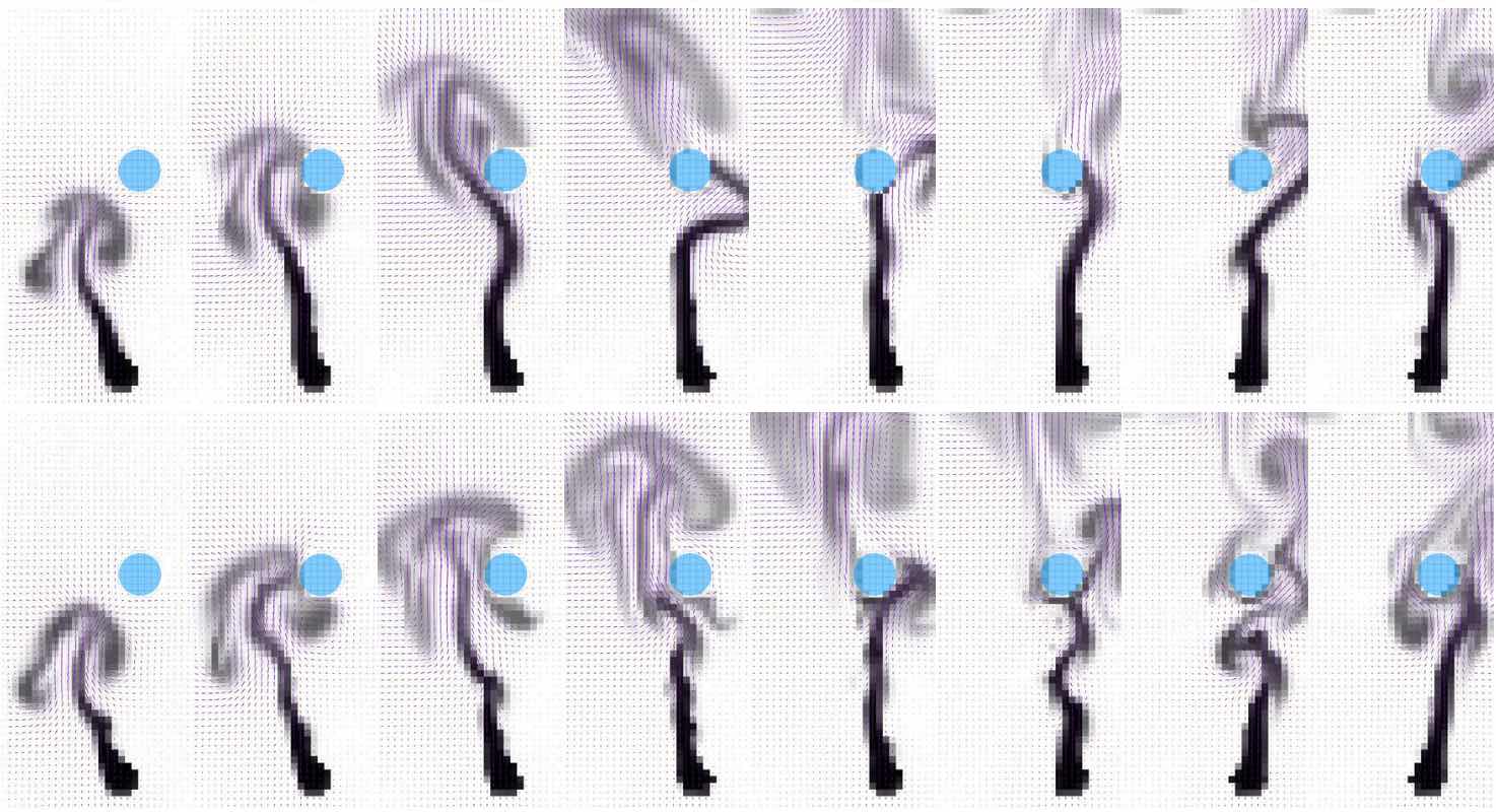
Fig. 59 The learned prediction is shown at the top, the reference simulation at the bottom.#
To summarize, DL allows us to move from linear subspaces to non-linear manifolds, and provides a basis for performing complex steps (such as time evolutions) in the resulting latent space.
Source code#
In order to make practical experiments in this area of deep learning, we can recommend this latent space simulation code, which realizes an end-to-end training for encoding and prediction. Alternatively, this learned model reduction code focuses on the encoding and decoding aspects.
Both are available as open source and use a combination of TensorFlow and mantaflow as DL and fluid simulation frameworks.